Fourier Transform Through The Concept of Sampling
Fourier Transform Overview
Have you ever tried to identify the ingredients in a delicious smoothie? It can be tough to tell how much milk, water, or veggies are in there, right? Well, imagine that smoothie is actually a signal, and we need to break it down into its individual components. That’s where the Fourier Transform comes in. It’s a powerful tool that helps us decompose signals in the time domain into multiple frequency components. In other words, it can help us identify how each ingredient contributes to the overall taste of the smoothie.
The Fourier Transform is not only useful for analyzing signals, but it’s also helpful for solving difficult problems that might be impossible to solve in the time domain alone. By viewing signals in different domains, we can gain insights and solve problems that might have otherwise been out of reach.
Mathematically, the Fourier Transform involves taking a signal in the time domain1 and transforming it into the frequency domain. This transformation reveals the various frequencies present in the signal, allowing us to better understand and analyze it. The Fourier Transform is widely used in fields such as audio and image processing, communications, and medical imaging, to name just a few.
By understanding the Fourier Transform, we can gain insights into the complex signals that surround us and use this knowledge to solve problems and create innovative solutions.
Mathematically, Fourier Transform is defined as
\(\begin{equation} X(f)= \mathcal{F}\{x(t)\} = \int_{-\infty}^{\infty} x(t)e^{-2\pi ift} dt \label{eq:inverse} \tag{1} \end{equation}\)
\[\begin{equation} x(t)= \mathcal{F} \{X(f)\} = \int_{-\infty}^{\infty} X(f)e^{2\pi ift} df \label{eq:forward} \tag{2} \end{equation}\]The mathematical definition of the Fourier Transform can look quite intimidating at first glance, but it’s actually quite simple. Equation \eqref{eq:inverse}, known as the forward Fourier Transform, shows that by applying some math to a continuous function \(x(t)\) in the time domain, we can obtain the frequency information \(X(f)\). Equation \eqref{eq:forward}, known as the inverse Fourier Transform, does the opposite: it takes frequency information and converts it back into the time domain.
While these equations are the generalized cases, there are actually several variants of the Fourier Transform, including Fourier Series, Discrete-time Fourier Series, Discrete-time Fourier Transform, and Discrete Fourier Transform. Each variant has its own set of equations, making it challenging to remember them all. That’s why this post will provide an intuitive, logical way to understand the Fourier Transform without having to remember every equation.
One way to understand the Fourier Transform is through the concept of sampling. Imagine you have a signal that varies over time, such as a sound wave. To analyze this signal, you can sample it at regular intervals and record the amplitude of the signal at each sample point. This creates a discrete representation of the original signal, which can be transformed into the frequency domain using the Fourier Transform.
By using sampling, we can break down a signal into its component frequencies and analyze each one separately. This is useful for a wide range of applications, from audio processing to image compression. In the next section, we’ll explore this concept in more detail and provide some examples to help you understand how the Fourier Transform works in practice.
Sampling
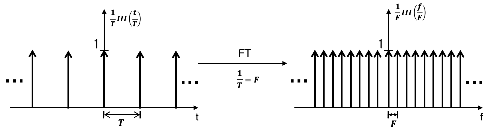
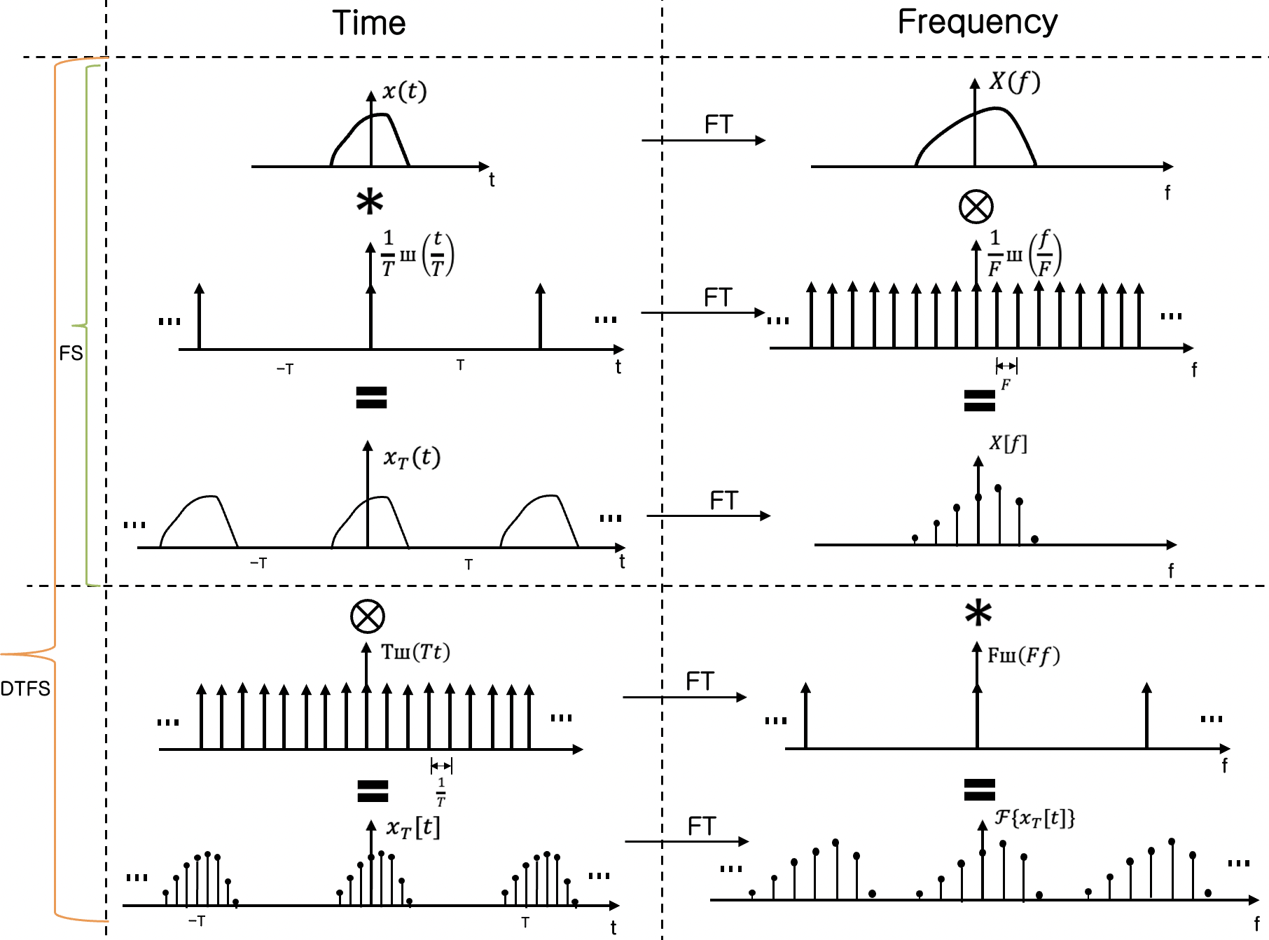
To better understand how the Fourier Transform works, we’ll start with the dirac comb function (can also be called shah function, impulse train), which is an essential concept in sampling. The Dirac comb is a periodic function with a period of \(T\), defined as follows:
\[\begin{equation} ш_{T}(t)=\int_{-\infty}^{\infty}\delta(t - kT)\\ = \frac{1}{T}ш(\frac{1}{T}) \label{eq:diraccomb} \tag{3} \end{equation}\]In this formula, \(\delta(t)\) is the impulse function, and \(ш(t)\) denotes a dirac comb with a unit period. The dirac comb function is important in sampling because it allows us to convert a continuous signal into a discrete signal by sampling it at regular intervals.
One interesting property of the dirac comb function is that its Fourier Transform is another dirac comb, but with a period that is the multiplicative inverse of its counterpart in the time domain. This means that if the dirac comb has a period of \(T\) in the time domain, its Fourier Transform will have a period of \(1/T\) in the frequency domain.
Sampling is a crucial process for converting continuous-time signals into discrete-time signals that can be processed by computers. In simple terms, sampling involves extracting values from a continuous-time signal at regular intervals to create a sequence of discrete-time values that represent the original signal.
To perform sampling, we use the dirac comb function to multiply the continuous-time signal. This creates a series of impulses at regular intervals, which we can then use to extract discrete-time values from the signal. Mathematically, this can be represented as follows:
\[\begin{equation} x[t]=\frac{1}{T}ш(\frac{1}{T}) x(t) \label{eq:sampling} \tag{4} \end{equation}\]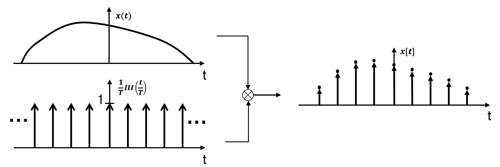
At this point, it is encouraged to keep in mind the 2 mantras that are the building blocks for everything that comes later
-
Fourier Transform of a dirac comb is also a dirac comb \(\mathcal{F}\{\frac{1}{T}ш(\frac{t}{T})\} = {\frac{1}{F}ш(\frac{t}{F})}\) for \(T=\frac{1}{F}\)
-
Convolution in time domain \(<=>\) multiplication in the frequency domain and vice versa
By keeping these principles in mind, we can gain a deeper understanding of the Fourier transform and its many variants, which we’ll explore in the upcoming sections.
Fourier Series
In this section, we will dive into the Fourier Series and its properties. Consider a finite continuous signal \(x(t)\) and its periodic extension \(x_T(t)\) with a period \(T\). The question arises, what does the Fourier transform of a periodic signal look like? Is it also periodic and continuous in the frequency domain? Can we grasp these concepts intuitively without delving into the math?
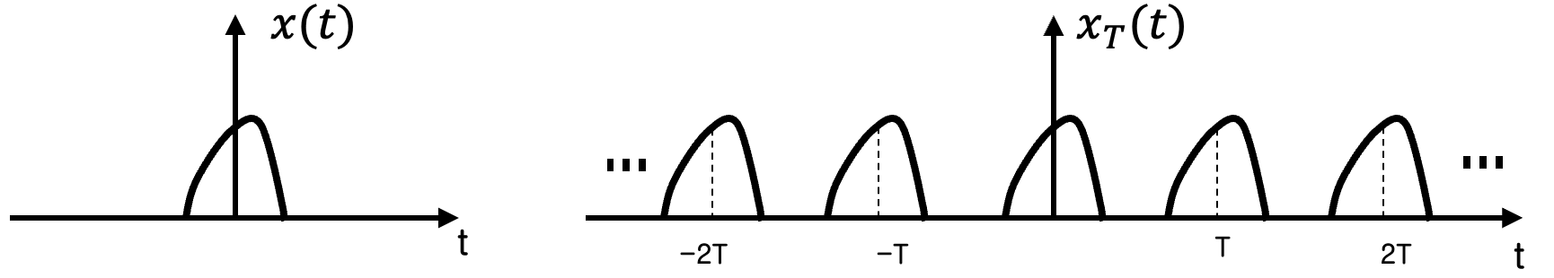
While it may not be immediately informative to look at the signal \(x_T(t)\) alone, we can gain a deeper understanding by breaking it down into smaller units. It’s worth noting that \(x_T(t)\) is just the convolution of \(x(t)\) and the dirac comb function \(\frac{1}{T}ш(\frac{t}{T})\).
\[\begin{equation} x_T(t)=\frac{1}{T}ш(\frac{t}{T})*x(t) \label{eq:5} \tag{5} \end{equation}\]Remember the two important properties discussed earlier: Fourier Transform of a dirac comb is also a dirac comb, and convolution in the time domain is equivalent to multiplication in the frequency domain. Applying these properties to the frequency domain, we obtain
\[\begin{equation} X [f] = \frac{1}{F}ш(\frac{t}{F})X(f) \label{eq:6} \tag{6} \end{equation}\]where \(\mathcal{F}\{x_T(t)\} = X[f]\) and \(\mathcal{F}\{x(t)\} = X(f)\).
It turns out that this is exactly the form of sampling (equation \eqref{eq:sampling}). The only difference is that signal is now sampled in the frequency domain instead of the time domain.
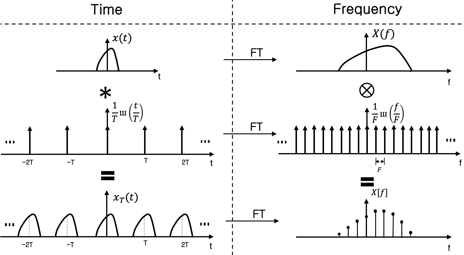
The big picture is that Fourier Transform of a continuous periodic signal \(x_T(t)\) is a discrete sequence that is the sampling of \(X(f)\) at rate \(F=\frac{1}{T}\) in the frequency domain. \(x_T(t)\) can be written as the sum of sine and cosine waves using Fourier Series.
\[\begin{equation} x_T(t) = \sum_{n=-\infty}^{\infty} c_{n}e^{ in \omega_{0} t} \label{eq:fs} \tag{7} \end{equation}\] \[\begin{equation} c_{n} = \frac{1}{T} X[n \omega_{0}] \label{eq:cn} \tag{8} \end{equation}\]where \(c_{n}\) is called Fourier Transform coefficient representing the height of the corresponding frequency component, \(\omega_{0} = 2 \pi f_{0}\) and \(f_{0}\) is the fundamental frequency \(f_{0} = \frac{1}{T}\).
Expressing periodic signals in the form of Fourier Series using complex exponentials is useful for calculations because complex exponentials are the eigenfunctions of the Linear Time-Invariant (LTI) system. However, this concept goes beyond the scope of this post.
Discrete-Time Fourier Series
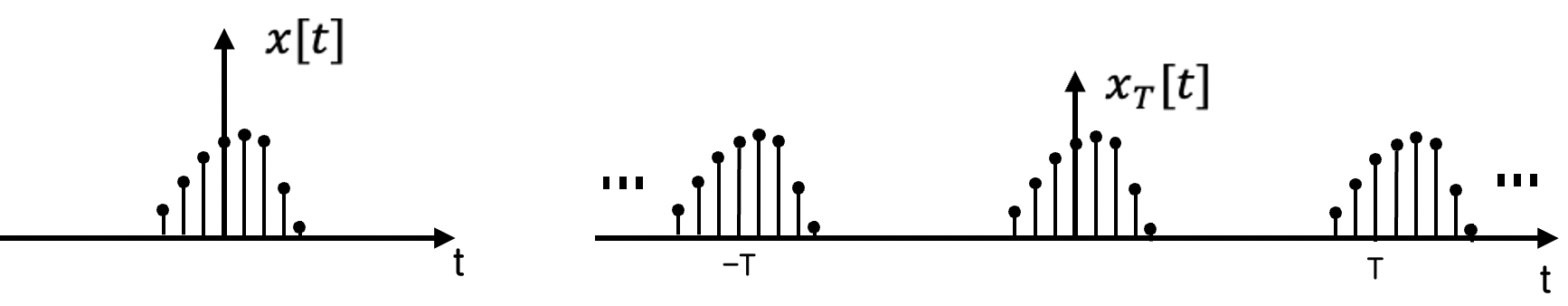
The title says it all. This time, we consider a periodic discrete-time signal (whereas previously it’s periodic continuous-time). We have a finite discrete function \(x[t]\), and \(x_T[t]\) is the periodic extension of \(x[t]\) with period \(T\).
Again, we’re gonna see the problem from the sampling point of view.
\(x_T[t]\) can be expressed as
\[\begin{equation} x_T[t] = x(t) * \frac{1}{T}ш(\frac{t}{T}) . Tш(Tt) \label{eq:dtfs1} \tag{9} \end{equation}\]Mapping into frequency domain (again, using the two mantras)
\[\begin{equation} \mathcal{F}\{x_T[t]\} = \mathcal{F}\{x(t)\} . \mathcal{F}\{\frac{1}{T}ш(\frac{t}{T})\} * \mathcal{F} \{Tш(Tt)\} \\ = X(f) . \frac{1}{F}ш(\frac{f}{F}) * Fш(Ff) \\ = X[f] * Fш(Ff) \label{eq:dtfs2} \tag{10} \end{equation}\]Therefore, \(\mathcal{F}\{x_T[t]\}\) is Fourier Transform of continuous periodic signal \(x_T(t)\) duplicated infinite times.
Likewise, \(x_T[t]\) can also be written in the form of a Fourier Series
\[\begin{equation} x_T[t] = \sum_{n=-\infty}^{\infty} c_{n}e^{ in \omega_{0} t} \label{eq:dtfs} \tag{11} \end{equation}\] \[\begin{equation} c_{n} = \frac{1}{T} X[n \omega_{0}] \label{eq:dtfs_cn} \tag{12} \end{equation}\]Conclusion
To summarize, in this post, we’ve started by defining what is Fourier Transform at a high level. It is followed by discussing how to use the lens of sampling to intuitively crack the code of some variants of Fourier Transform — Fourie Series (FS) and Discrete-Time Fourier Series (DTFS). Let’s explore some other variants on the next one.
-
not necessarily in time domain but let’s just simply assume the time-frequency duality here. ↩
Comments