A Friendly Guide to Flow Matching in Deep Learning
Flow Matching has been generating significant buzz in the AI community lately. This innovative technique is poised to replace the highly successful Diffusion modeling and has already been integrated into cutting-edge models like Stable Diffusion 3, Resemble Enhance, and E2TTS. Intrigued by its potential, I decided to delve into the world of Flow Matching to understand how exactly it works in theory and practice.
Over the past few weeks, I immersed myself in learning about the concept of Flow Matching. While the journey was enjoyable, the concept proved to be quite abstract and challenging to understand. In this blog post, I aim to demystify Flow Matching and present it in a straightforward manner that anyone can follow. I hope someone would find this useful!
Update: I recently applied Flow Matching to my area of expertise—Speech Synthesis. If you’re interested in seeing how it works in this context, check out my detailed exploration here.
Diffusion Recap and Motivation of Flow Matching
Most of us are probably somewhat familiar with the concept of the diffusion process in diffusion-based models. Let’s refresh real quick.
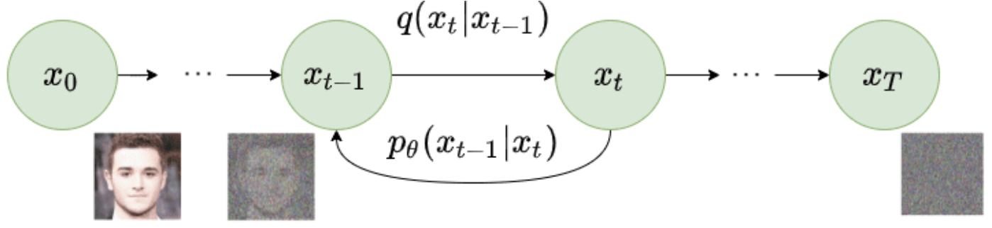
In the forward diffusion process, noise is incrementally added to a data point over multiple steps. If enough steps are taken, the data point eventually transforms into complete noise. Conversely, the reverse diffusion process systematically denoises the noisy data point in multiple steps, reconstructing the original input.
Now, you might wonder: why do we need to specify processes to add and remove noise from data? Why not adopt a more general approach, where the goal is simply to transform a simple distribution (typically a Gaussian) into a target distribution? As long as we can find a way to get to target distribution, we’re good! This broader perspective is the motivation behind Flow Matching. We’ll delve into the details in the upcoming sections.
Flow Matching
Before diving into the concept of Flow Matching (FM), let’s define the foundational components that build the FM framework.
Probability Density Path (p):
\[[0,1] \times \mathbb{R}^d \rightarrow \mathbb{R} (>0)\]Unlike a regular probability distribution, a probability density path is time-dependent (with time ranging from \(0\) to \(1\)). At any given time and location, it provides the probability density of that specific location at that particular time. In deep learning,
\(p_0\) (the distribution at \(t=0\)) is a simple distribution, such as a Gaussian, while \(p_1\) (the distribution at \(t=1\)) represents the dataset distribution we aim to model.
Vector Field (v):
\[[0,1] \times \mathbb{R}^d \rightarrow \mathbb{R}^d\]This constructs a flow \(\phi\) defined by the Ordinary Differential Equation (ODE)
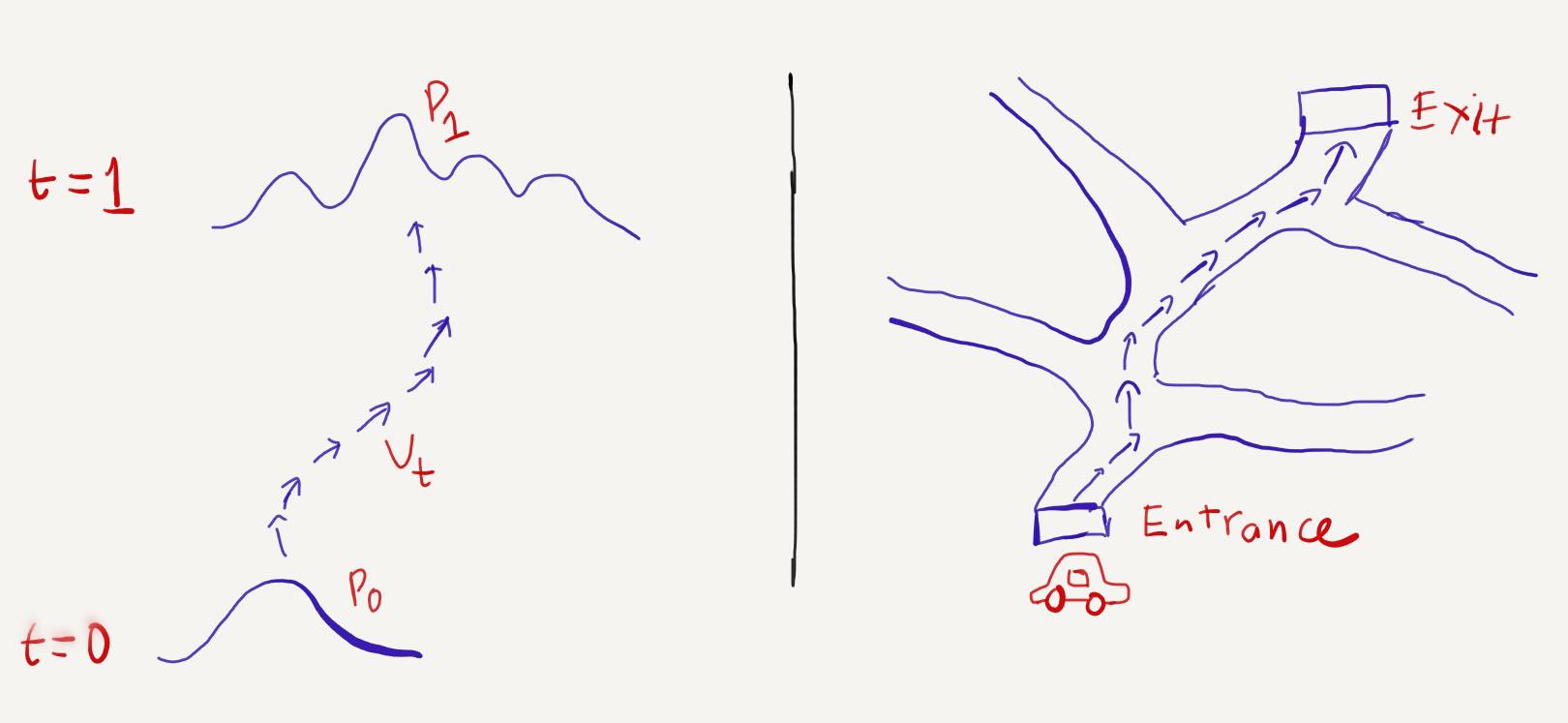
\[\frac{d}{dt} \{ \phi_t(x) \} = v_t(\phi_t(x))\] \[\phi_0(x) = x\]The flow \(\phi\) pushes \(p_0\) along the time dimension so that at \(t=1\), the probability density becomes \(p_1\). This is represented by the push-forward equation:
\[p_t = [\phi_t] * p_0\]To transition from a source distribution \(p_0\) to a target distribution \(p_1\), we need to understand the flow of the probability path. According to the ODE equation, \(\phi_t\) is constructed by \(v_t\). Therefore, to determine \(\phi_t\), we only need to find \(v_t\).
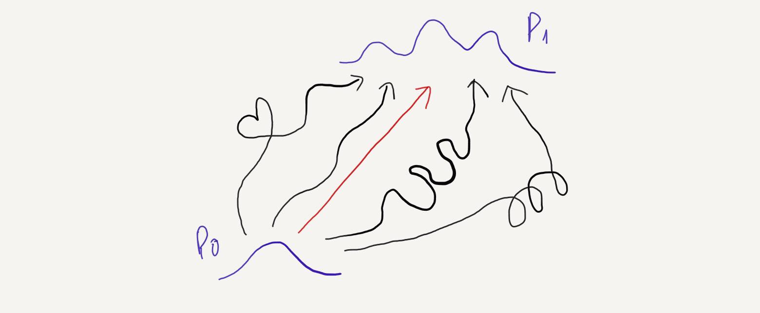
If this still feels abstract, imagine driving a car on a highway for the first time without prior knowledge of how to reach the exit. You start at the entrance (\(p_0\)) and follow a series of small arrows (\(v_t\)) painted on the road, guiding you to the exit (\(p_1\)).
Now, let \(x_1\) denote a random variable distributed according to the approximate data distribution \(p_1\), with \(p_0\) being a simple distribution like a Gaussian. As mentioned, \(v_t\) determines the probability path and the flow. If we know \(v_t\), we can transform \(p_0\) into \(p_1\). In other words, knowing \(v_t\) allows us to model the data distribution \(p_1\).
The Flow Matching objective is:
\[L_{FM}(\theta) = E_{t, p_t(x)} ||v_t(x) - u_t(x)||^2\]where \(v_t(x)\) is the “ground truth” vector field, and \(u_t(x)\) is the estimated vector field from a neural network. Simply put, FM loss minimizes the difference between the vector field \(v_t\) and the predicted \(u_t\).
While this might seem straightforward, there’s a significant problem: the FM objective is intractable. We don’t have a closed form for \(v_t\) and \(p_t\), which are what we’re trying to find. The solution to this issue is a method called Conditional Flow Matching.
Conditional Flow Matching
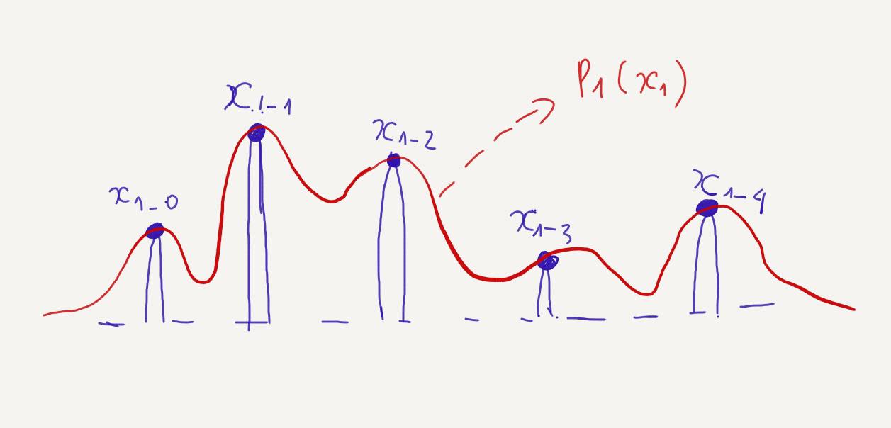
Given a dataset with \(N\) datapoints \((x_{1_0}, x_{1_1}, x_{1_2}, \ldots, x_{1_N})\), it is nearly impossible to model the exact distribution of the dataset. However, we can approximate it by considering it as a mixture of simpler distributions.
We design a conditional probability distribution \(p_1(x \mid x_1)\) at \(t=1\) to be concentrated around \(x=x_1\). For instance, \(p_1(x \mid x_1)\) can be a normal distribution with mean \(x_1\) and a very small standard deviation \(\sigma\), such as \(p_1(x \mid x_1) = N(x \mid x_1, \sigma^2I)\). The overall distribution \(p_1(x)\) is then approximately a mixture of all these conditional probability distributions centered around each datapoint in the dataset.
The marginal probability \(p_1(x)\) is represented as
\[p_1(x) = \int p_1(x \mid x_1)q(x_1) \, dx_1\]Similarly, we can represent the probability path by marginalizing over the condition \(x_1\):
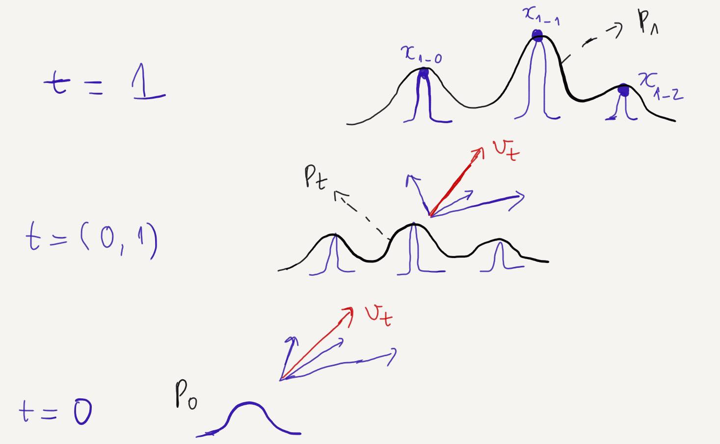
\[p_t(x) = \int p_t(x \mid x_1)q(x_1) \, dx_1\]We can also define the vector field \(v_t\) by marginalizing over the conditional vector fields:
\[p_t(x) = \int u_t(x \mid x_1)\frac{p_t(x \mid x_1) q(x_1)}{p_t(x)} \, dx_1\]This implies that while we don’t have a closed form for \(v_t\), we can approximate it by aggregating all the conditional vector fields \(v_t(. \mid x_1)\) according to all the datapoints.
So now we have the objective of CFM
\[L_{CFM}(\theta) = E_{t, p(x_1), p_t(x \mid x_1)} ||v_t(x \mid x_1 ) - u_t(x)||^2\]where \(t \sim U[0, 1], x_1 \sim p(x_1)\), and now \(x \sim p_t(x \mid x_1)\).
Unlike the FM objective, the CFM objective is tractable. We can sample from \(p_t(x \mid x_1)\) and compute \(v_t(x \mid x_1)\), both of which can be easily done as they are defined on a per-sample basis. So now we’re ready to train a CFM model with this objective, right? Well, not quite! If you notice, \(p_t(x \mid x_1)\) only specifies a probability path that somehow flows from \(p_0\) to the dataset distribution. However, there are countless possible paths that can flow from \(p_0\) to \(p_1\). Consequently, there are also countless possible vector fields. So among these infinite paths, which one should we use in practice? Let’s dive into the next part to figure it out.
CFM in practice
When training a Conditional Flow Matching (CFM) model, we can use any shape or type of probability path. Ideally, the modeling capability remains the same regardless of the chosen path, meaning the model can theoretically reach the global optimum with any path. However, in practice, we prefer using a straight-line probability path for several reasons:
- Faster model convergence
- Fewer steps needed during inference to achieve the same quality, resulting in faster inference
The most commonly used type of CFM, at least at the time of writing, is Optimal Transport Conditional Flow Matching (OTCFM). In OTCFM, the conditional probability path and the conditional vector field are defined as:
\[p_t(x) = N(tx_1 + (1 - t)x_0, t(t - 1)\sigma^2)\] \[u_t(x) = x_1 - x_0\]The straight-line probability path is represented by the mean \(\mu = tx_1 + (1 - t)x_0\) of \(p_t\). When \(t\) is close to \(0\), \(x_t\) is close to \(x_0\), and when \(t\) is close to \(1\), \(x_t\) is close to \(x_1\). At any time between \([0,1]\), \(\mu\) is the interpolation of \(x_1\) and \(x_0\).
Below is the backbone of OTCFM in semi-pseudo code if you ever wanna train a OTCFM model
import torch

# optimal transport conditional flow matching loss
class OTCFMLoss(nn.Module):
    def __init__(self):
        super(OTCFMLoss, self).__init__()
    def forward(self, ut, vt):
        loss_otcfm = torch.mean((vt - ut) ** 2)
        return loss_otcfm

# optimal transport conditional flow matching
class OTCFM(nn.Module):
    def __init__(self,
                 sigma=0.0001
                 ):
        super(OTCFM, self).__init__()

        self.sigma = sigma
        self.estimator = Estimator()
        self.timestep_embedding = Time_Embedding()
        self.conditioning_timestep_integrator = NN()
        self.xt_and_emb_integrator = NN()

        self.loss_otcfm = OTCFMLoss()

    def forward(self, x1, cond):
        """
        x1 <float> (B, D, T) –> Target
        cond <float> (B, D, T) –> conditioning - optional
        """
        B, D, T = x1.shape
        t = torch.rand(
            (B, 1, 1), dtype=x1.dtype, device=x1.device, requires_grad=False)

        # spherical gaussian noise
        x0 = torch.randn_like(x1)

        # interpolation between t-scaled x0 and x1
        xt = (1 - (1 - self.sigma) * t) * x0 + t * x1

        # interpolation between x1 and sigma scaled x0
        vt = x1 - x0 * (1 - self.sigma)

        time_emb = self.timestep_embedding(t[:, 0, 0])

        # intergrading conditioning and time embedding
        cond = self.conditioning_timestep_integrator(cond, time_emb)

        # integrating xt and cond
        x = self.xt_and_emb_integrator(xt, cond)

        ut = self.estimator(x)

        loss_otcfm = self.loss_otcfm(ut, vt)

        return loss_otcfm
After training, we obtain a neural network (estimator) that can estimate the vector field. So, what’s next? How do we perform inference with this estimator and the predicted vector field? The answer lies in using a Solver to solve the numerical integration of the Ordinary Differential Equation (ODE). There are several types of solvers available for ODEs, with one common method being the Euler method. Below is a semi-pseudo inference code using the Euler method:
    @torch.inference_mode()
    def inference(self, cond, n_steps=10):

        xt = torch.randn_like(...)  # same size as x1 in forward()
        t_span = torch.linspace(0, 1, n_steps + 1, device=xt.device)

        t, _, dt = t_span[0], t_span[-1], t_span[1] - t_span[0]

        for step in tqdm(range(1, len(t_span)), desc="Processing steps"):
            time_emb = self.timestep_embedding(t[:, 0, 0])

            # intergrading conditioning and time embedding
            cond = self.conditioning_timestep_integrator(cond, time_emb)

            # integrating xt and cond
            x = self.xt_and_emb_integrator(xt, cond)

            ut = self.estimator(x)

            dphi_dt = ut

            # ODE - using Euler method
            xt = xt + dt * dphi_dt
            t = t + dt

            if step < len(t_span) - 1:
                dt = t_span[step + 1] - t

        return xt
Conclusion
Flow Matching represents a significant advancement in deep learning, offering a more flexible and efficient approach to modeling complex data distributions. By understanding the principles behind Diffusion models, Flow Matching, and Conditional Flow Matching, we can appreciate the innovation and potential of these techniques. Through practical implementation, such as using the Euler method for inference, Flow Matching becomes a powerful tool in the AI toolkit. I hope this guide has provided you with a clear and approachable understanding of Flow Matching and its applications. Keep learning!
Comments